Model setup
Contents
- 1 Model setup for fracture flow and transport in limestone aquifers - steps
- 1.1 Conceptualization and setup of a conceptual model including geology and hydrogeology
- 1.2 Formulation of the modeling objectives
- 1.3 Choice of model complexity and modeling scale
- 1.4 Data acquisition - measurements to obtain relevant model parameters (see list of parameters for each model)
- 1.5 Delineation of the model domain based on physically meaningful boundaries (f.e. head isolines, no-flow boundaries)
- 1.6 Implementation of parameters for selected units in the model domain (homogeneous/heterogeneous)
- 1.7 Choice of boundary conditions for the flow and the transport model
- 1.8 Setup of sources and sinks: Definition of wells
- 1.9 For transient models: definition of initial conditions
- 1.10 Mesh generation
- 1.11 Simulation
- 1.12 Critical evaluation of the modeling results
- 1.13 Formulation of mass balances to check the model
- 1.14 Model calibration and validation
- 1.15 Model reporting
- 2 Flow chart giving an overview of the individual steps
- 3 Example: Setup of models for a contaminated site with a fractured limestone aquifer (Akacievej, Hedehusene)
Model setup for fracture flow and transport in limestone aquifers - steps
This chapter gives step-by-step instructions for the setup of a model to simulate flow and transport in a fractured limestone aquifer. The following describes the typical steps to setup a model for contaminant transport in a fractured limestone aquifer:
Conceptualization and setup of a conceptual model including geology and hydrogeology
Geologic modeling
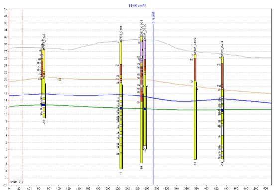
Boreholes can give valuable information about the geology.
Bits of geologic knowledge can be connected to establish a geologic model, that shows different geologic layers, to which properties can be assigned, and other relevant geologic information.

Formulation of the modeling objectives
Choice of model complexity and modeling scale
Based on available data and modeling objectives, the model complexity has to be chosen. A very complex and detailed model is not appropriate if only little field data is available. Then, a simple model can be applied, which can be refined as soon as new data is measured.
The modeling was an integrated part of the limestone project. Initially, a rough model based on first measurements and available data was setup and then used to plan further field work and measurements.
The scale is also depending on the modeling objectives. Source zone remediation needs a different scale than the risk assessment of a contaminant plume for water works. The following scales can be considered:
- well scale
- source zone scale
- intermediate scale for e.g. pumping tests
- plume scale
Data acquisition - measurements to obtain relevant model parameters (see list of parameters for each model)
Delineation of the model domain based on physically meaningful boundaries (f.e. head isolines, no-flow boundaries)
Implementation of parameters for selected units in the model domain (homogeneous/heterogeneous)
Choice of boundary conditions for the flow and the transport model
Setup of sources and sinks: Definition of wells
For transient models: definition of initial conditions
Mesh generation
When working with complex models it is useful to start with a coarse mesh to test the model and the setup with limited time effort. For the real simulations, a finer grid can be employed. Modern grid generators allow a mesh refinement at specific parts of the mesh. Especially at heterogeneities and fractures and at concentration fronts, the mesh should be sufficiently fine to resolve gradients appropriately. This can be tested by a grid refinement study, where the mesh is refined and the results are compared. When the solution does not change with a grid refinement, it is sufficiently resolved.
Simulation
Critical evaluation of the modeling results
Modeling results should be always critically evaluated and tested. It is for example helpful, to have a check the mass balance of a model. It is also important to have a general look at the results, by . f.e. visualizing the hydraulic heads or concentrations in the entire domain. Then, it can be checked, if the boundary conditions are fulfilled and if there are any disturbances in the model domain.
Formulation of mass balances to check the model
Model calibration and validation
Model reporting
Flow chart giving an overview of the individual steps
ADD FLOW CHART
Example: Setup of models for a contaminated site with a fractured limestone aquifer (Akacievej, Hedehusene)
The setup of a discrete-fracture model in 2D in COMSOL Multiphysics is described in the following document:
The typical workflow for modeling a contaminated site will be demonstrated using an example field site close to Copenhagen.
Example: Setup of models for a field site (Akacievej, Hedehusene)
Return to Content