Steps to setup a model for flow and transport in fractured limestone aquifers
This chapter gives an overview of the recommended steps to setup a model for the simulation of flow and transport in a fractured limestone aquifer.
The following list shows the typical steps to setup a model for contaminant transport in a fractured limestone aquifer.
Expand an item (button on the right) to get more information about it.
Formulation of the modeling objectives
Before setting up a model, it is important to define the specific modeling objective(s).
The choice of the model concept, model extent, modeling scale and included details should be closely linked to these objectives.
One should aim at including the most relevant features in the model, while keeping it as simple as possible to address the modeling objective(s).
The following list gives some examples for modeling objectives:
- Delineate the capture zone of a well
- Improve risk assessment, e.g. for a contaminant threatening a drinking water well, in order to assess future actions
- Analyze the distribution and potential spreading of a contaminant plume in an aquifer
- Test hypotheses related to the origin of a contaminant
- Interpret observed / measured field data
- Analyze the influence of transient hydraulic conditions (annual variations, pumping in the area) on plume propagation
- Develop and optimize a remediation strategy for the source zone of a contaminated site
- Optimize a remediation strategy for a contaminant plume
Conceptualization and setup of a conceptual model including geology and hydrogeology
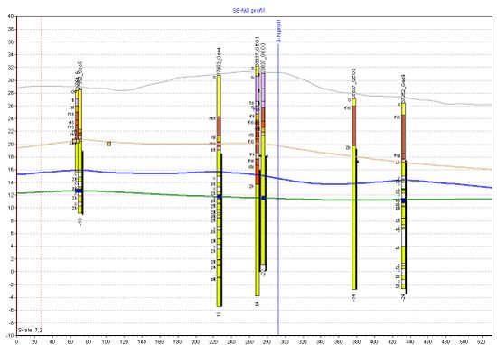 Example geologic profile of a Geoscene3D model. Geologic modeling
Borehole data, outcrops, geophysical measurements etc. can give valuable information about the geology at a site.
Bits of geologic knowledge can be connected to establish a geologic model, that shows different geologic layers and relevant geologic features (like inclusions or lenses).
Typically, these layers are characterized by different hydrogeologic properties.
The geometry can be stored as a CAD interpolation of the surfaces, that delineate the geologic layers.
Tools like GeoScene3D can be very useful to manage borehole data and to create interpolation surfaces.
The surfaces can be imported into the numerical model later on.
Definition of the model scope
The scale also depends on the modeling objectives.
The model scope will, for example, be different for the prediction of the spreading of an entire plume (large scale) and for the planning of source zone remedial actions (local scale).
An important aspect when choosing the model extent is to have the boundaries sufficiently far away from the most influential features in the area, such as pumping wells.
The model extent has to be big enough, so that the boundaries do not influence the results in the area of interest.
It should be chosen based on physically meaningful boundaries (f.e. known head isolines or no-flow boundaries).
The modeling of source zone remediation requires a different scale than the risk assessment of a contaminant plume for water works.
The following scales can be distinguished:
- well or borehole scale
- source zone scale
- intermediate scale for e.g. pumping tests
- plume scale
Based on available data and modeling objectives, the model complexity has to be chosen.
A very complex and detailed model is not appropriate if only little field data is available.
Then, a simple model can be applied, which can be improved as soon as new data is measured.
Modeling was an integral part in the limestone project and already done at an early stage of the project.
Initially, a rough model based on first measurements and available data was setup.
It was used for the planning of further field work and measurements.
It also helps to identify further data requirements and to plan measurements that support the modeling.
These additional measurements and data can then be incorporated in the model.
Data acquisition - measurements to obtain relevant model parameters (see list of parameters for each model)
Implementation of parameters for selected units in the model domain (homogeneous/heterogeneous)
Based on available data and the chosen model, parameter distributions have to be defined.
For a steady-state flow simulation, the hydraulic conductivity (or permeability) is required.
For transport, parameters like porosity, (effective) diffusion coefficients, dispersivities and sorption parameters are required.
Choice of boundary conditions and sources/sinks
Boundary conditions should be chosen according to known or delineated boundaries, such as geologic boundaries, known hydraulic head isolines, known flowlines (can be used as no-flow condition perpendicular to them, if the flow field is stable).
The most common boundary conditions are
- Dirichlet conditions (or first-type boundary conditions), where the primary variable is fixed to a value (e.g. fixed hydraulic head or fixed concentration).
- Neumann conditions (or second-type boundary conditions), where the gradient of the primary variable is specified (e.g. flux across the boundary, often no-flow boundaries)
- Cauchy conditions (or third-type boundary conditions), which sets a condition to the primary variable and its derivative (used f.e. for the infiltration flux through a river bed).
The proper choice of boundary conditions is a very important step and determines the calculated results.
Sources and sinks can be added in the model domain to include e.g. withdrawal/injection at wells or groundwater recharge due to precipitation.
For transient models: definition of initial conditions
Steady-state models do not require the definition of initial conditions.
Transient problems, however, require to specify the initial value of the primary variables (e.g. concentrations at each location of the model domain.
Mesh generation
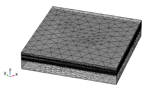 Example a mesh used for discrete-fracture simulations of the Akacievej tracer tests. The mesh is refined at the horizontal fractures and at the wells. When working with complex models it is useful to start with a coarse mesh to test the model and the setup with limited computational efforts.
When the model is properly setup, a finer grid can be employed.
Modern grid generators allow a local mesh refinement at specific locations in the model domain.
Locations, where strong gradients of the primary variables (head, concentration) occur, should be resolved at a high resolution, while for the parts of the model domain with only small changes, a coarser mesh resolution may be sufficient.
Especially at heterogeneities and fractures, at wells and at concentration fronts, the mesh should be sufficiently fine to resolve the local gradients (e.g. of concentration or head gradients) appropriately.
If the applied mesh is sufficiently fine can be tested by a grid refinement study, where the mesh is gradually refined and the model results are compared.
When the results do not significantly change with a further grid refinement, the grid resolution is sufficient.
Simulation
After setting up the geometry, boundary conditions, initial conditions, material parameters and simulation parameters (simulation time, solver settings), the actual simulation can be run.
It is always a good idea to start with a test run, f.e. with a coarse mesh and a short duration, to test if everything is set as desired.
Critical evaluation of the modeling results
Modeling results should always be critically evaluated and the model should be properly tested.
It is, for example, helpful, to check the mass balance of a model, i.e. to balance all inflows and outflows and the storage in the model domain.
It is also important to visually inspect the results, f.e. by visualizing the hydraulic heads and concentrations in the domain and in special areas of interest.
Then, it should be checked, if the results look reasonable and as expected, if the boundary conditions are fulfilled and if there are any disturbances like oscillations in the model domain.
Oscillations can be an indication for a too coarse mesh.
It is also a good idea to test for grid convergence, i.e. to test if the model results change, when the numerical grid is refined.
Model calibration and validation
more information will be included soon
Model reporting
more information will be included soon
Example: Setup of a COMSOL Multiphysics model for a contaminated site with a fractured limestone aquifer (Akacievej, Hedehusene)
The setup of a discrete-fracture model in 2D in COMSOL Multiphysics using Coefficient Form PDEs is described in the following document:
COMSOL provides also the possibility to include fracture flow in the Darcy's Law interface, while fracture transport can be included in the Transport of Diluted Species in Porous Media interface.
We refer to the product documentation for more details.
FEFlow provides a tutorial, that describes the steps of setting up a flow and transport model and how to include discrete fractures.
DRAFT: The typical workflow for modeling a contaminated site will be demonstrated using an example field site close to Copenhagen.
Example: Setup of models for a field site (Akacievej, Hedehusene)
Return to Content
|

